41. Semi-supervised learning
How to use a lot of un-labeled data with a few labels effectively?
Introduction
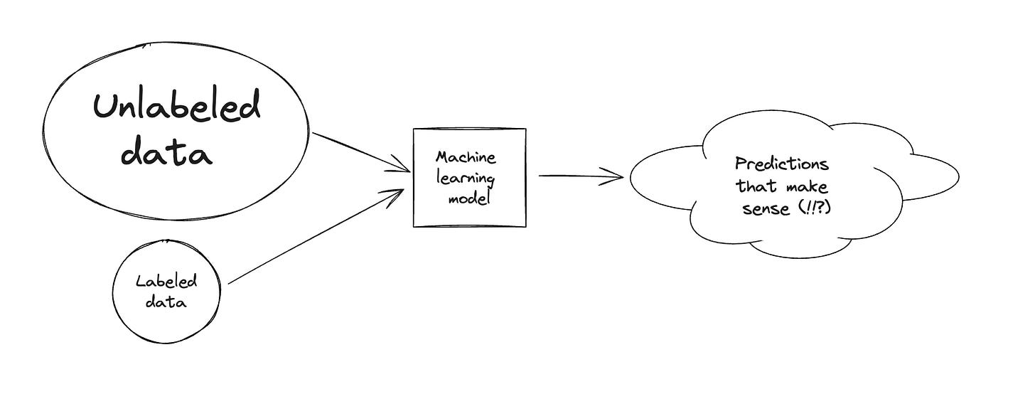
Semi supervised learning is halfway between supervised and unsupervised learning.
In addition to unlabelled data, the algorithm is provided with some supervision information - but not necessarily for all examples!
The labeled portion is usually quite small compared to to the unlabeled one…!
The objective is to leverage unlabeled examples to train a better performing model than what can be obtained using only the labeled portion of the dataset.
In general, we can see the loss function made up of two components:
Where:
… that is not very interesting. Let’s focus on the other term which is made up of a weighting term that increases the importance of the unlabeled loss and the loss itself.
The semi supervised techniques we are going to see today are all going to focus on the second term:
Consistency regularization
Temporal ensembling
Mean teachers
Pseudo labeling
Label propagation
Self training
Before exploring the techniques, a few assumptions on the data we are dealing with:
Smoothness Assumptions: If two data samples are close in a high-density region of the feature space, their labels should be the same or very similar.
Cluster Assumptions: The feature space has both dense regions and sparse regions. Densely grouped data points naturally form a cluster. Samples in the same cluster are expected to have the same label.
Low-density Separation Assumptions: The decision boundary between classes tends to be located in the sparse, low density regions.
Manifold Assumptions: The high-dimensional data tends to locate on a low-dimensional manifold. Even though real-world data might be observed in very high dimensions (e.g. such as images of real-world objects/scenes), they actually can be captured by a lower dimensional manifold where certain attributes are captured and similar points are grouped closely (e.g. images of real-world objects/scenes are not drawn from a uniform distribution over all pixel combinations).
Very loosely: assume data can be grouped together nicely and that data lives on a low enough dimensional space even if it looks like that’s not the case!
With that out of the way, let’s explore a few techniques you can employ in your day job to fix all your label issues (the most common machine learning problem is lacking proper labels!)
Techniques
Consistency regularization
This technique assumes that randomness within the model (have you heard of Dropout?) or data augmentation transformations should not modify model predictions given the same input.
Then, as unlabeled loss you can pick a consistency regularization loss!
As an example, you could minimize the difference between two passes through the network with stochastic transformations. The label is not explicitly used in this setting!
Temporal ensembling
In the technique above, we doubled the cost of training because we run two passes per sample. To reduce the cost, we can maintain an exponential moving average of the model prediction in time per training sample as the learning target.
This moving average is updated only once per epoch.
Mean teachers
Temporal Ensembling keeps track of an EMA of label predictions for each training sample as a learning target. However, this label prediction only changes every epoch, making the approach clumsy when the training dataset is large.
Instead of tracking the moving average of model outputs, we can track the moving average of model weights.
The model with the moving average weights is the mean teacher model which provides more accurate results.
The consistency regularization loss is the distance between predictions of the student and teacher models.
Pseudo labeling
Pseudo Labeling assigns fake labels to unlabeled samples based on the maximum softmax probabilities predicted by the current model and then trains the model on both labeled and unlabeled samples simultaneously in a pure supervised setup.
“How does this even work??” - you might ask.
Well, it is proven this is equivalent to entropy regularization.
You can also see this technique naturally as a teacher student model again as it is an iterative process again: the model that produces pseudo labels is teacher and the model that learns with pseudo labels as student.
Label propagation
Label Propagation is an idea to construct a similarity graph among samples based on feature embedding.
Then the pseudo labels are “diffused” from known samples to unlabeled ones where the propagation weights are proportional to pairwise similarity scores in the graph.
This technique is conceptually similar to a k-NN classifier and both suffer from the problem of not scaling up well with a large dataset.
Self training
Self-Training is an iterative algorithm, alternating between the following two steps until every unlabeled sample has a label assigned:
Initially it builds a classifier on labeled data.
Then it uses this classifier to predict labels for the unlabeled data and converts the most confident ones into labeled samples.
One critical element in their setup is to have noise during student model training but have no noise for the teacher to produce pseudo labels.
Noise is important for the student to perform better than the teacher. The added noise has a compound effect to encourage the model’s decision making the frontier smooth on both labeled and unlabeled data.
A few other important technical configs in noisy student self-training are:
The student model should be sufficiently large (i.e. larger than the teacher) to fit more data.
Noisy student should be paired with data balancing, especially important to balance the number of pseudo labeled images in each class.
Soft pseudo labels work better than hard ones.
Conclusions
I hope you can employ these techniques at your current job to make your ML models shine bright with impact! :)


